
The presentation of this paper led me to think that the model TRANSYT uses for priority situations may not be fully understood.
Firstly, let me explain, briefly, how we suggest (but not insist) a priority approach is dealt with on a signalised roundabout. To begin with, the coefficient and max flow needs to be deduced. The easiest way of achieving this is by using ARCADY. Enter all the geometric details of the junction under consideration and you will obtain a value for the yintercept (the max flow in TRANSYT) and the slope (the coefficient in TRANSYT). It is necessary to know how ARCADY works to do this, of course. Having deduced the parameters for the priority approach this way, it is necessary to specify which link is to oppose the entry traffic. For this it is important to use just one link to model all the traffic that has priority. This may seem odd at first because you may be modelling two or more traffic streams, or lanes, and if the approach was signalled, you would need more than one link. However, using a single link is acceptable in this situation because it is unsignalled and we are not interested in how queues form and discharge: only the pattern of traffic as it passes the priority arm is needed. If it is necessary to model different movements on this link you can still use shared links, and you can use them to model different lanes if necessary in this case (but don’t even think of doing that on any signal controlled approaches!) Specify the master link as the priority link in the give-way data.
When the priority model has been specified, it is important to appreciate how it works. The relationship that is given by the give-way parameters is used in each step of the cycle, separately, to calculate the potential flow out of the give-way arm during each step. Thus, when there is little traffic on the circulating link, there should be (potentially) more flow getting out of the give-way link (assuming that there is traffic demand present). Conversely, when there is a larger flow on the circulating link, there is a limit to what can enter. This way a new cyclic profile is built up from the circulating and entry profiles to feed downstream links. The new profile will generally look like the circulating profile with the gaps filled in.
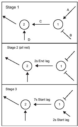 Figure 1 – Stage sequence
What the method above doesn’t necessarily consider is the way upstream signals affect traffic behaviour, especially when long intergreens are injected to produce gaps that allow downstream give-way traffic to enter. When this is the case, it is likely that the give-way traffic can see that upstream traffic has been halted, anticipate the impending gap, and be able to discharge across the give-way line, almost as if it was a signal controlled stopline. Under these circumstances, it may be worth considering Stuart Maxwell’s method as an alternative to the normal give-way model. But the consideration has to be careful and the way to model it needs some additional explanation. Below I have suggested a method that should cover all eventualities. It is not the only way, but it combines give-way and signalled parameters.
In the diagrams below, arms (or phases) A and B (see Figure 1) are the circulating and entry arms at a signal controlled junction 1. These feed arm C which is a signal controlled arm associated with node 1 (not 2). D is in fact a bottleneck link and node 2 doesn’t actually exist in the TRANSYT data. However, this bottleneck link also gives way to arm C. Now we can specify signal data on arm C that makes it red for the induced gap and arm D will use the specified standard saturation flow value during that period. The rest of the time, arm D will use the give-way parameters, with the (usually) lower maximum flow.
Figure 2 shows the timings to use when the journey time between nodes 1 and 2 is 7 seconds and the induced gap is 5 seconds (the time that A and B are both red). Both need to be adjusted to model each situation. Note that the example deals with the situation when there is one induced interstage. If there are to be two periods, simply insert another all-red stage in the way illustrated, using the second-green facility to model phases A and B.
The main advantages of this method is that both the normal priority situation and the alternative ‘neo signal controlled’ situation are both modelled together, in an automatic fashion. It can be used to set the intergreen length to the minimum required, and allow a more accurate model of platoons further downstream. Make sure that you use the cyclic flow profile graphs to see how the model is working and adjust the lags and all-red time as necessary.
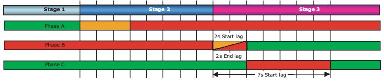
Figure 2 – Timings for a 7 second induced gap